Can we look-up and return multiple values in one cell in Excel (separated by comma or space)? I have been asked this question multiple times by many of my colleagues and readers. Excel has some amazing lookup formulas, such as VLOOKUP, INDEX/MATCH (and now XLOOKUP), but none of these offer a way to return multiple matching values. All of these work by identifying the first match and return that. So I did a bit of VBA coding to come up with a custom function (also called a User Defined Function) in Excel. In this tutorial, I will show you how to do this (if you’re using the latest version of Excel – Microsoft 365 with all the new functions), as well as a way to do this in case you’re using older versions (using VBA). So let’s get started!
Lookup and Return Multiple Values in One Cell (Using Formula)
If you’re using Excel 2016 or prior versions, go to the next section where I show how to do this using VBA. With Microsoft 365 subscription, your Excel now has a lot more powerful functions and features that are not there in prior versions (such as XLOOKUP, Dynamic Arrays, UNIQUE/FILTER functions, etc.) So if you’re using Microsoft 365 (earlier known as Office 365), you can use the methods covered in this section could look up and return multiple values in one single cell in Excel. And as you will see, it’s a really simple formula. Below I have a data set where I have the names of the people in column A and the training that they have taken in column B.
Click here to download the example file and follow along For each person, I want to find out what training they have completed. In column D, I have the list of unique names (from column A), and I want to quickly lookup and extract all the training that every person has done and get these in a single set (separated by a comma). Below is the formula that will do this:
After entering the formula in cell E2, copy it for all the cells where you want the results. How does this formula work? Let me deconstruct this formula and explain each part in how it comes together gives us the result. The logical test in the IF formula (D2=$A$2:$A$20) checks whether the name cell D2 is the same as that in range A2:A20. It goes through each cell in the range A2:A20, and checks whether the name is the same in cell D2 or not. if it’s the same name, it returns TRUE, else it returns FALSE. So this part of the formula will give you an array as shown below: {TRUE;FALSE;FALSE;TRUE;FALSE;FALSE;FALSE;FALSE;FALSE;FALSE;FALSE;FALSE;FALSE;FALSE;FALSE;FALSE;FALSE;FALSE;FALSE} Since we only want to get the training for Bob (the value in cell D2), we need to get all the corresponding training for the cells that are returning TRUE in the above array. This is easily done by specifying [value_if_true] part of the IF formula as the range that has the training. This makes sure that if the name in cell D2 matches the name in the range A2:A20, the IF formula would return all the training that person has taken. And wherever the array returns a FALSE, we have specified the [value_if_false] value as “” (blank), so it returns a blank. The IF part of the formula returns the array as shown below: {“Excel”;””;””;”PowerPoint”;””;””;””;””;””;””;””;””;””;””;””;””;””;””;””} Where it has the names of the training Bob has taken and blanks wherever the name was not Bob. Now, all we need to do is combine these training name (separated by a comma) and return it in one cell. And that can easily be done using the new TEXTJOIN formula (available in Excel 2019 and Excel in Microsoft 365) The TEXTJOIN formula takes three arguments:
the Delimiter – which is “, ” in our example, as I want the training to separated by a comma and a space character TRUE – which tells the TEXTJOIN formula to ignore empty cells and only combine ones that are not empty The If formula that returns the text that needs to be combined
If you’re using Excel in Microsoft 365 that already has dynamic arrays, you can just enter the above formula and hit enter. And if you’re using Excel 2019, you need to enter the formula, and hold the Control and the Shift key and then press Enter Click here to download the example file and follow along
Get Multiple Lookup Values in a Single Cell (without repetition)
In case there are repetitions in your data set, as shown below, you need to change the formula a little bit so that you only get a list of unique values in a single cell.
In the above data set, some people have taken training multiple times. For example, Bob and Stan have taken the Excel training twice, and Betty has taken MS Word training twice. But in our result, we do not want to have a training name repeat. You can use the below formula to do this:
The above formula works the same way, with a minor change. we have used the IF formula within the UNIQUE function so that in case there are repetitions in the if formula result, the UNIQUE function would remove it. Click here to download the example file
Lookup and Return Multiple Values in One Cell (Using VBA)
To get multiple lookup values in a single cell, we need to create a function in VBA (similar to the VLOOKUP function) that checks each cell in a column and if the lookup value is found, adds it to the result. Here is the VBA code that can do this: Where to Put this Code? How does this formula work? This function works similarly to the VLOOKUP function. It takes 3 arguments as inputs: 1. Lookupvalue – A string that we need to look-up in a range of cells. 2. LookupRange – An array of cells from where we need to fetch the data ($B3:$C18 in this case). 3. ColumnNumber – It is the column number of the table/array from which the matching value is to be returned (2 in this case). When you use this formula, it checks each cell in the leftmost column in the lookup range and when it finds a match, it adds to the result in the cell in which you have used the formula.
Remember: Save the workbook as a macro-enabled workbook (.xlsm or .xls) to reuse this formula again. Also, this function would be available only in this workbook and not in all workbooks. Click here to download the example file
Get Multiple Lookup Values in a Single Cell (without repetition)
There is a possibility that you may have repetitions in the data. If you use the code used above, it will give you repetitions in the result as well. If you want to get the result where there are no repetitions, you need to modify the code a bit. Here is the VBA code that will give you multiple lookup values in a single cell without any repetitions. Once you have placed this code in the VB Editor (as shown above in the tutorial), you will be able to use the MultipleLookupNoRept function. Here is a snapshot of the result you will get with this MultipleLookupNoRept function.
Click here to download the example file In this tutorial, I covered how to use formulas and VBA in Excel to find and return multiple lookup values in one cell in Excel. While it can easily be done with a simple formula if you’re using Excel in Microsoft 365 subscription, if you’re using prior versions and don’t have access to functions such as TEXTJOIN, you can still do this using VBA by creating your own custom function.
How to Create and Use an Excel Add-in. How to Run a Macro in Excel. Find the Last Occurrence of a Lookup Value a List in Excel How to Use VLOOKUP with Multiple Criteria How to Record a Macro in Excel – A Step by Step Guide. Test Multiple Conditions Using Excel IFS Function
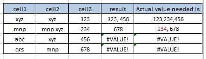
list2 PRODUCT55,OP513N16,PROODUCT61,OP495G74 ——————————————> 1 OP512E08,PRODUCT31,PRODUCT48,PRODUCT19,OP513N16 ————————> 2 PRODUCT43,OP495G74,PRODUCT22,OP747B38,PRODUCT74,PRODUCT23—–> 3 EXPECTED RESULTS 2,1,2 3 1,3 i ’d like lookup about all parts of list1 in all list2 but results of every cell be in one cell as the expected results thank u Thanks a lot. thanks Thanks a lot for this solution. But would there be an option that it checks each cell in (not only column A) lets say the A+B+C column and that it will return me the value of column D? Thanks, I tried to use this formula and it works great. But i have a question: Would it be possible that not only the values from collum C will be returned but also of for example values from Collum D and E? Thanks for your help, Can anyone please help me getting this work. Thanks!!! Your VBA code is fantastic and its serving my purpose to a great extent. But i am facing another problem which needs to solved. Please help me with the coding. Problem is in the desired ColumnNumberi.e result column some cells are blank. So your code is accepting the blank value(with a delimiter) along with other values. Below example will clear the problem: Col A Col B Col C Col D (Sales Person) ( Products) (Sales Pearson) (Result) 1 Superman Toy Superman Toy, , Staionery 2 Spiderman Spiderman , , Toy 3 Batman Stationery Batman Stationery, Toy, Soap 4 Krishh Grocery Krishh Grocery, ,Soap 5 Superman 6 Spiderman Grocery 7 Batman Toy 8 Krishh 9 Superman Stationery 10 Spiderman Toy 11 Batman Soap 12 Krishh Soap So it’s similar to your code, but looks along a row, instead of down a column. Thanks We have used a code for only one column or a cell as a lookup reference. Now I need to include one more to this. 2 columns as s lookup reference to get the same results. My code as per your example code is below. Function SingleCellExtractInward(lookupvalue As String, lookuprange As Range, ColumnNumber As Integer) Dim i As Double Dim Result1 As String Dim Result2 As String If Result2 = Empty Then Result2 = “no recent inward” SingleCellExtractInward = Result2 End If For i = 1 To lookuprange.Columns(1).Cells.Count If lookuprange.Cells(i, 1) = lookupvalue Then Result1 = Result1 & ” ” & lookuprange.Cells(i, ColumnNumber) & “,” SingleCellExtractInward = Left(Result1, Len(Result1) – 1) End If Next i End Function Could you please help me on this code to lookup 2 columns as a reference.? I have included it into my macro enabled spreadsheet and everytime it executes there is a compile error, like the one mentioned by Laura below. Compile Error: Syntax Error SingleCellExtract = Left(Result, (Len(Result) – 1)) I have tried altering the brackets but no improvement. It looks like it cannot find the added function but I am just guessing. Any suggestions? Could it be a setting local to me on I think the example xlsm down load is fine but the above code text included some funny error in the call to SingleCellExtract = Left(Result, Len(Result) – 1) It seems there is a funny character in there after copy / paste. As I just deleted it and typed it by hand and then it was fine. Really pleased as does exactly what I need. Function SingleCellExtract(Lookupvalue As String, LookupRange As Range, ColumnNumber As Integer) Dim i As Long Dim Result As String For i = 1 To LookupRange.Columns(1).Cells.Count If LCase(LookupRange.Cells(i, 1)) = LCase(Lookupvalue) Then Result = Result & ” ” & LookupRange.Cells(i, ColumnNumber) & “,” End If Next i SingleCellExtract = Left(Result, Len(Result) – 1) End Function for example: https://uploads.disquscdn.com/images/72b430f0123fb5f1ca1275477c73ded853c901e314ec1f7da59821b316c02e9d.jpg Can we get code to reverse this function i have multiple HCodes like H310, H302, etc in one column & corrosponding statement in another column like corrosive for these two codes can i get a code to do v lookup for different h code in same cell saperated by coma to their corrosponding statement without repetation for example if two h codes having same statement i get on statement Lokesh I am trying to use this macro, but I get the below error: Compile Error: Syntax Error and it highlights the below portion, as the step it get stuck on SingleCellExtract = Left(Result, Len(Result) – 1) My data is 3 columns, my formula goes as follows: =SingleCellExtract(E3,$A:$C,3) E3 is the value (a number) i want it to find in the range $A:$C is the range 3 is the 3rd column where i want the formula to look to pull out the results (result is text). What am i doing incorrectly? Another great idea from you. Code optimised and options integrated Public Function fLookUpMultiple(ByRef LookUpValue As String, _ ByRef LookUpRange As Excel.Range, _ ByRef ColumnNumber As Long, _ Optional ByRef bUnique As Boolean = True) As String ‘Variant ‘Get all values from a list that match specific value Dim lgRow As Long Dim strFilter As String Dim lgElement As Long For lgRow = 1 To LookUpRange.Columns(1).Cells.Count If bUnique Then If LookUpRange.Cells(lgRow, 1).Value2 = LookUpValue Then For lgElement = 1 To lgRow – 1 If LookUpRange.Cells(lgElement, 1).Value2 = LookUpValue Then If LookUpRange.Cells(lgElement, ColumnNumber).Value2 = LookUpRange.Cells(lgRow, ColumnNumber).Value2 Then GoTo Skip End If Next lgElement strFilter = strFilter & ” ” & LookUpRange.Cells(lgRow, ColumnNumber) & “,” Skip: End If Else If LookUpRange.Cells(lgRow, 1).Value2 = LookUpValue Then strFilter = strFilter & ” ” & LookUpRange.Cells(lgRow, ColumnNumber).Value2 & “,” End If Next lgRow ‘Delete last “,” fLookUpMultiple = VBA.Left(strFilter, VBA.Len(strFilter) – 1) End Function It does what you are looking for, and uses a data validation drop down instead of a combo box. But it can be easily replicated for a combo box as well. Hope this helps! To get values without duplicates, use this code: Function SingleCellExtract(Lookupvalue As String, LookupRange As Range, ColumnNumber As Integer) Dim i As Long Dim Result As String For i = 1 To LookupRange.Columns(1).Cells.Count If LookupRange.Cells(i, 1) = Lookupvalue Then For J = 1 To i – 1 If LookupRange.Cells(J, 1) = Lookupvalue Then If LookupRange.Cells(J, ColumnNumber) = LookupRange.Cells(i, ColumnNumber) Then GoTo Skip End If End If Next J Result = Result & ” ” & LookupRange.Cells(i, ColumnNumber) & “,” Skip: End If Next i SingleCellExtract = Left(Result, Len(Result) – 1) End Function
