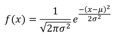
Where μ (mu) is the mean and σ (sigma) is the standard deviation.
Normal Distribution Probability Density Function in Excel
It’s also referred to as a bell curve because this probability distribution function looks like a bell if we graph it. It’s a well known property of the normal distribution that 99.7% of the area under the normal probability density curve falls within 3 standard deviations from the mean. So to graph this function in Excel we’ll need a series of x values covering (μ-3σ,μ+3σ). This is the probability density function for the normal distribution in Excel.
Graphing the Normal Probability Density Function
We can graph the normal probability density function in Excel by setting up a table with two columns of values.
X – This is a series of real numbers that will appear on our X-axis which we will evaluate our normal density function on.f(X) – This is the result of our normal density function evaluated at X.
If we select our table then go to the Insert tab and select a Line Chart from the Charts section. We can see the result is a nice bell shaped curve centered around the mean value.
Create a Normally Distributed Set of Random Numbers in Excel
Is it possible to create a set of normally distributed values in Excel? Yes, it is, but we will need to look at the cumulative distribution function F(x)=P(X<=x) and it’s inverse function. This is the probability that a random value from the distribution is less than a given value x. The formula involves calculus but thankfully Excel’s NORM.DIST function will do this calculation for us.
We can also graph this in a similar manner to the probability density function and create a Line Chart from the Charts section of the Insert tab. Note that the Y-axis of this chart goes from 0 to 1. This is a probability value and represents the probability of a random value from our normal distribution being less than or equal to a given value. As an example F(0)=50% so there’s a 50% chance a random value from our normal distribution will be below 0. From this graph, we can also start with a probability on the Y-axis and get a value from our normal distribution on the X-axis. This is call the inverse of a function. If we start at 0.8 on the Y-axis and follow out horizontally until we hit the graph, then move vertically down we will arrive at the 0.788 on the X-axis. This means 0.788 is the inverse of 0.8. Using the inverse function is how we will get our set of normally distributed random values. We will use the RAND() function to generate a random value between 0 and 1 on our Y-axis and then get the inverse of it with the NORM.INV function which will result in our random normal value on the X-axis.
If we do this calculation 1,000 times we can graph it with a Histogram chart and we start to see a bell shape curve emerge.
With 10,000 values, the distribution becomes more clear.
In fact because of the law of large numbers, the more of these randomly generated normal values we create, the closer our graph will appear bell shaped.
Box Muller Method to Generate Random Normal Values
The Box-Muller method relies on the theorem that if U1 and U2 are independent random variables uniformly distributed in the interval (0, 1) then Z1 and Z2 will be independent random variables with a standard normal distribution (mean = 0 and standard deviation = 1).
We will easily be able to create these formulas in Excel with U1=RAND() and U2=RAND(). For our purposes though, we will only need to calculate Z1. Since Z1 will have a mean of 0 and standard deviation of 1, we can transform Z1 to a new random variable X=Z1*σ+μ to get a normal distribution with mean μ and standard deviation σ.
We can also graph this with a Histogram for a large number of calculations and see a nice well defined bell shaped curve.